Take a position (first 2–3 sentences)
Most visual inspection pilots die not because the model failed but because teams mis-estimated labeling cost and the ongoing cost of false positives. If you treat a CV pilot like a research experiment, you will burn budget; treat it like a manufacturing system and you win — fewer defects, fewer line stops, dollars saved.
Minimum viable dataset: how many defect examples do you actually need
Short answer: start by sizing for the defect class complexity and prevalence, not a magic number. In our production work the difference between a ship-or-fail pilot is whether you budgeted for 200–2,000 true defect examples per class and disciplined negative sampling.
Practical rules of thumb
- Simple, high-contrast defects (scratches, single missing screw): 200–500 defect images per class often gets you to a deployable model with >90% precision in controlled lighting.
- Moderate complexity (shape deformations, multiple failure modes): 1,000–3,000 defect images per class to reach stable recall across parts and fixtures.
- High variability (cosmetics across many SKUs, reflective surfaces): 5,000+ defect images and frequent domain adaptation.
Table: defect-example guidance
| Defect complexity | Typical defect examples per class | When to scale further |
|---|---|---|
| Simple / high contrast | 200–500 | Poor generalization across camera angles |
| Moderate / texture or occlusion | 1,000–3,000 | Multiple SKUs/fixtures require per-SKU sampling |
| High / reflective, variable lighting | 5,000+ | Use synthetic augmentation + domain adaptation |
Why prevalence matters
If defects are 0.1% of parts on the line, collecting 1,000 defect images requires sampling ~1M parts — expensive and slow. Instead: (a) seed a targeted collection plan using controlled fault injection / seeded defects, (b) use vendor-assisted synthetic augmentation for small defects, and (c) instrument a short closed-loop labeling pipeline after go-live to collect the long tail.
Measureable milestone: aim for a validation set with at least 100 held-out true defect examples per class that reflect production lighting and line speed — that gives you actionable validation metrics without optimism bias.
Labeling tradeoffs: class labels, bounding boxes, pixel masks, and negative sampling
Labeling cost is where most projects blow budgets. Choose the minimal label that supports the decision on the line.
- Decision-first labeling: label what the downstream action needs. If the line only needs "pass/reject", binary or polygonal labels suffice. If localizing a rework spot is required, use bounding boxes or instance masks.
- Bounding box vs mask: masks increase label time 2–4×. Use masks only when precise localization changes your rework cost materially.
- Per-defect class vs aggregated defect: separate classes only when repair or handling differs; otherwise group into a single "reject" class and add metadata.
- Negative sampling: a labeled negative set is critical. A 10:1 negative:positive sampling ratio in the training set prevents models from learning spurious cues (background, fixture markings).
Labeling quality rules
- Use toolchains with annotation QA and consensus labels (Roboflow, Vatic-style workflows, commercial labeling platforms). Expect median label speed: 1–3 minutes per bounding box depending on complexity.
- Budget 20–30% of data costs for QA re-annotation on a random 5% sample.
Triage labeling spend: spend heaviest on rare/high-cost defects. If a defect causes a 30% scrap cost, prioritize accurate labels and more samples for that class.
Expected on-line accuracy and validation rig
Be explicit about the metric that matters: recall (catch defects) vs precision (avoid false rejects). On-line economics usually prioritize recall up to a tolerable false reject rate.
Typical on-line ranges we see when a project is executed as a production system (controlled lighting, fixed camera, engineering-led DA):
- Simple defects: precision 95–99%, recall 90–98%.
- Moderate defects: precision 90–97%, recall 80–95%.
- High variability: precision 85–95%, recall 70–90% until you add domain adaptation.
Validation rig (must-do)
- Deploy a shadow mode on-line for 2–4 weeks: record model decisions and human outcomes without blocking the line.
- Capture per-SKU, per-shift, per-camera metrics; stratify by conveyor speed and fixture.
- Build an automated example stream for hard-failures: any missed defect gets a priority slot for re-label and model retrain.
ASCII pipeline (useful deployment diagram)
Camera -> Edge preprocess (crop/normalize) -> Inference (Edge GPU/TPU) -> Decision logic
                 |                             |                     |
                 v                             v                     v
          Local logging -----------------> Shadow logs --------> MLOps retrain loop
Log enough context with each image: SKU, camera ID, timestamp, conveyor speed, human disposition.
Inference options and deployment tradeoffs 🔌
Pick hardware for budget and latency. You will see models run on NVIDIA Jetson (Xavier/NX), Google Coral (Edge TPU), and cloud accelerators like AWS Inferentia. Choose based on throughput, power, and maintainability.
Comparison table
| Option | Typical throughput | Power | Ease of ops | Best for |
|---|---|---|---|---|
| NVIDIA Jetson Xavier NX | 30–200 FPS (depends on model) | 10–30W | Medium (containerized) | Complex models, PyTorch/TensorRT |
| Google Coral (Edge TPU) | 30–150 FPS (quantized models) | 2–4W | Easy (TFLite) | Simple/quantized classifiers |
| AWS Inferentia (cloud) | Very high (parallel instances) | N/A | High (managed) | Centralized inference, high throughput |
| AWS Panorama | Variable (edge appliance + camera) | Appliance-level | Managed integration | Deployable CAM-to-cloud with Panorama SDK |
Vendor stacks: pick a product you can operate. Landing AI is strong for data-centric model iteration and domain adaptation; Cognex / ViDi suits tightly integrated factory hardware workflows; Roboflow is useful for fast labeling and augmentation; AWS Panorama pairs well with Inferentia if you already run on AWS. We prefer TensorRT optimized models on Jetson for latency-critical lines and TFLite/Coral when power is constrained.
Mid-market ROI calculator: cost per avoided defect and run-rate savings
Formulae
- Cost avoided per defect = saved scrap/rework + avoided downstream costs (warranty, returns).
- Annual savings = defects avoided per year × cost avoided per defect − operating cost (inference, labeling amortized, maintenance).
Example (mid-market electronics line)
- Parts produced/year: 5,000,000
- Baseline defect rate: 0.2% (10,000 defects/year)
- Deployable model catch rate improvement: from 30% to 80% (additional 5,000 defects caught)
- Cost per defect avoided: $40 (scrap + rework + inspection downstream)
- Annual gross savings: 5,000 × $40 = $200,000
- Annual ops cost: edge HW amortized $30k + labeling/retrain $40k + infra $10k = $80k
- Net annual savings: $120k
- ROI year 1 = (Net / Ops) = 150% (payback < 1 year)
Use this quick calculator when prioritizing defect classes: rank by (defect frequency × cost per defect) / cost to collect labels. That ranking identifies the low-hanging fruit that funds the longer tail.
Where teams typically fail (and how to avoid it)
- Under-budget negative samples: you need many non-defect varieties; collect them early.
- Skipping shadow mode: you won’t see false-positive economics until the model is on-line.
- Over-labeling masks when boxes suffice: cuts speed and raises cost.
- Picking a vendor without deployment experience: name vendors (Landing AI, Cognex, Roboflow, AWS Panorama) and pick the one you already operate with.
Measure every change with dollars or uptime. Niche.dev treats a solution as real only when it has a number behind it: dollars saved, hours returned, defects caught, downtime cut.
Conclusion & CTA
If you want a practical plan — how many defect images to collect this quarter, what to buy for edge inference, and a simple ROI table for your finance team — start with a discovery that produces a labeled pilot spec and a 90-day collection plan.
Need help with visual inspection AI? Book a free strategy call with Niche.dev.
Niche.dev notes: we ship computer vision & detection systems (defect detection, PPE/safety vision) and MLOps for production AI. In past engagements we've delivered outcomes including PPE/safety vision that cut incidents by 75% and predictive maintenance that prevented $2.4M in equipment failures — use those outcomes as benchmarks when sizing impact.
Suggested Internal Links
- synthetic://cmouha5dg0000mh0fg9jxfbt2/indexed-content/niche-dev/mlops-enterprise.md
- synthetic://cmouha5dg0000mh0fg9jxfbt2/indexed-content/niche-dev/data-audit-ai.md
- synthetic://cmouha5dg0000mh0fg9jxfbt2/indexed-content/niche-dev/enterprise-ai-strategy.md